How we built a Knowledge Graph-powered NL2SQL agent

Natural language to SQL (NL2SQL) is one of those problems that sounds solved until you actually try to deploy it in production. Give an LLM your schema, a few examples, and ask it to write SQL, and it works, until it doesn’t. The bigger and messier your data warehouse, the faster the cracks appear.

This post walks through a different approach: instead of throwing raw schema at an LLM and hoping for the best, we built a knowledge graph layer that understands the semantic meaning of our warehouse. The result is a two-phase system, GraphRAG Pipeline, that routes questions through a structured graph before a single line of SQL is ever written.

Why traditional NL2SQL breaks at scale

To understand why we took this approach, it helps to understand where the research on NL2SQL currently stands, and where it keeps hitting walls.

The field has evolved through several distinct eras. Early rule-based systems like LUNAR required heavy manual feature engineering and couldn’t handle linguistic variety. Deep learning models (Seq2SQL, SQLNet) improved pattern recognition but still struggled with nested queries and cross-domain generalization. Pre-trained language models like BERT and TaBERT helped unify natural language and schema representations, but they needed domain-specific fine-tuning and explicit schema linking mechanisms to work well. Today’s LLMs, like GPT-4, Codex, and LLaMA, handle zero-shot and few-shot scenarios much more effectively, but they still hit a consistent set of walls:

• Schema complexity. When you dump a 200-table schema into a prompt, you’re spending most of your context window on tables that are completely irrelevant to the question. The model has to guess what’s relevant, and it frequently guesses wrong.
• Linguistic ambiguity. A query like “which category has the highest sales volume?” doesn’t map cleanly to table names. The gap between business language and database naming conventions is where most NL2SQL failures originate.
• Cross-domain fragility. Models trained or prompted on one domain often fail to generalize to another because schema structures, terminology, and join patterns differ so dramatically. 

Retrieval-Augmented Generation (RAG) addresses some of this by dynamically fetching relevant schema details rather than stuffing everything into a static prompt. But standard RAG (vector similarity search over schema metadata) still retrieves isolated text fragments. It doesn’t understand relationships between tables, and it can’t reason about join paths or semantic hierarchies.

That’s where Graph RAG enters the picture.

The core idea: Semantic routing through a Knowledge Graph

Recent research has formalized why graph-based retrieval is particularly well-suited to NL2SQL tasks. Unlike traditional semantic search methods that retrieve isolated textual snippets, Graph RAG constructs a structured knowledge graph that organizes entities, relationships, and schema components into an interconnected hierarchy. This matters because databases are inherently relational, and flat schema representations miss that entirely.

The core insight is this: schema is syntactic, but questions are semantic. A user asking about “sales volume by category” is reasoning in business concepts. The database stores this across a fact table and a dimension table, joined on a foreign key. A graph that explicitly maps the business concept to the physical tables and understands the join path between them makes this translation tractable and reliable.

Phase 1: Building the Knowledge Graph

This is the “build once” phase. The graph has three layers, each with a distinct purpose.

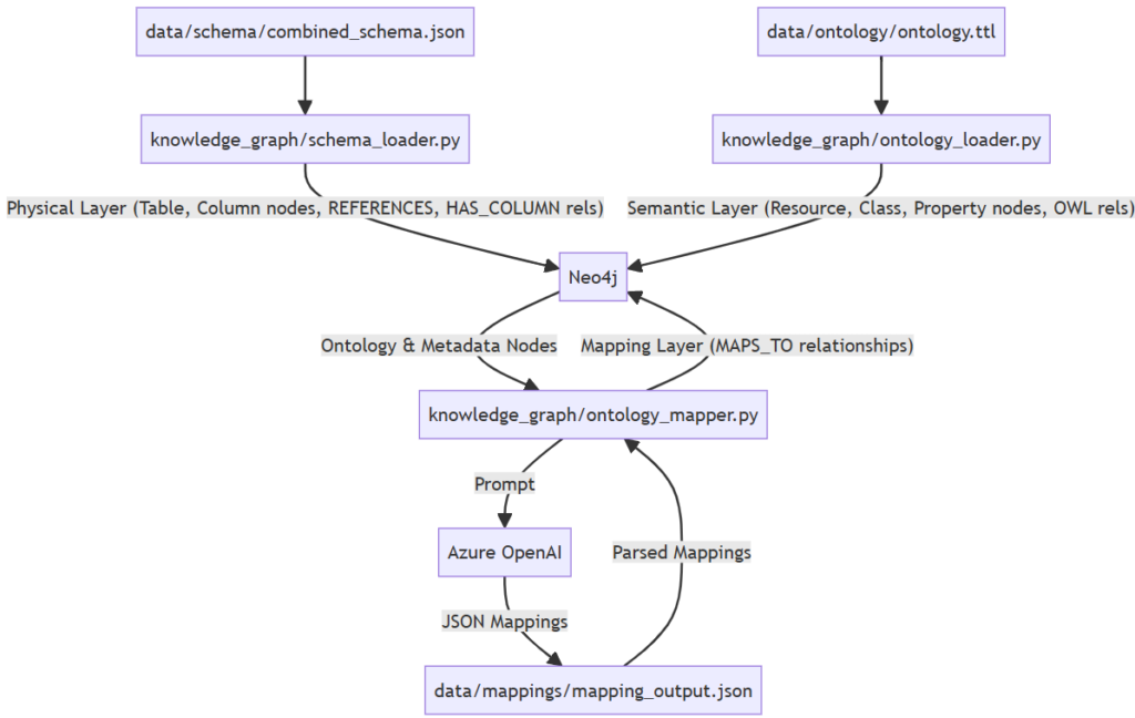
Layer 1: The physical layer

The physical layer mirrors your data warehouse structure. Using a combined_schema.json file that captures tables, columns, types, descriptions, and foreign key relationships, we load :Table and :Column nodes into Neo4j:

MERGE (t:Table {name: "fact_Sales"})
SET t.view_name = "[Reporting].[fact_Sales]",
    t.description = "Records transactional sales events."
​
MERGE (c:Column {table: "fact_Sales", name: "ProductID"})
SET c.sql_type = "INT", c.description = "FK linking to the product."
​
MERGE (t)-[:HAS_COLUMN]->(c)

Foreign key relationships become :REFERENCES edges, meaning the graph already understands how tables join together before any question is asked. This is the schema linking capability that RAG-based systems have been trying to improve: instead of the LLM inferring join paths from flat text, they’re explicitly encoded in the graph structure.

Layer 2: The Semantic layer (the OWL ontology)

This is where the architecture diverges most sharply from standard NL2SQL approaches. We define a domain ontology in OWL/Turtle that captures the business concepts of the warehouse:

:Sale
    a owl:Class ;
    rdfs:label   "Sale" ;
    rdfs:comment "Represents a recorded sales transaction." .
​
:hasProduct
    a owl:ObjectProperty ;
    rdfs:domain :Sale ;
    rdfs:range  :Product ;
    rdfs:label  "has product" ;
    rdfs:comment "Links a sale to the product involved." .

The ontology is deliberately rich. It’s not just a list of classes, but it also encodes the knowledge of the domain:

• Classes and properties: Sale, Product, Customer, CustomerReview etc., with relationships like inStock, submittedReview, hasFeature, etc.
• Business rules: What “customer engagement” means in this domain. What makes a product “underperforming.” Logic that lives in analysts’ heads, now expressed formally.
• Constraints: Opportunities have close dates; Products don’t. These prevent malformed queries before they reach SQL.
• Calculated metrics: Formulas for complex KPIs, so the LLM isn’t inventing aggregation logic from scratch.
• Disambiguation rules: When a term like “conversion” could mean a lead becoming an opportunity or a user becoming a paid subscriber, the ontology specifies which interpretation applies in which context.
• Synonyms: This is particularly valuable. Business users rarely use the exact language encoded in table names. The ontology maps synonyms explicitly.

:Sale
    a owl:Class ;
    rdfs:label   "Sale" ;
    rdfs:comment "Represents a recorded sales transaction." ;
    skos:altLabel "transaction", "order", "purchase", "deal" .
​
:Category
    a owl:Class ;
    rdfs:label   "Category" ;
    rdfs:comment "A product grouping used for reporting." ;
    skos:altLabel "segment", "product type", "vertical", "bucket" .

When a user asks about “deals by vertical,” the semantic decomposition step in Phase 2 can resolve “deals” to :Sale and “vertical” to :Category, not because the LLM guessed, but because the ontology explicitly encodes that mapping. This is the difference between a system that works for power users who know the schema and one that works for the broader business.

The ontology is loaded into Neo4j using the neosemantics (n10s) plugin, which imports Turtle files directly and creates :Resource, :Class, :Resource :ObjectProperty, and :Resource :DatatypeProperty nodes. The ontology can be LLM-generated from the schema metadata, but it requires human review before loading. Errors here propagate all the way through to query generation, so the manual review checklist before loading the TTL file isn’t optional, it’s the quality gate for the whole system.

Layer 3: The Mapping layer (the bridge)

The physical and semantic layers exist independently until the mapping layer connects them. This is the schema linking step, but done offline and systematically rather than at query time under pressure.

An LLM is given both the full ontology and the full schema and asked to produce typed, confidence-scored mappings:

{
  "ontology_node":  "https://ontology.example.io/insights#Sale",
  "metadata_node":  "fact_Sales",
  "mapping_type":   "CLASS_TO_TABLE",
  "confidence":     "HIGH",
  "reasoning":      "Sale class maps directly to fact_Sales transaction table."
}

Four mapping types are defined, covering the full range of relationships between business concepts and physical schema object.

Mapping type	When to use
CLASS_TO_TABLE	A dimension or fact table implements an OWL Class
DATATYPE_PROP_TO_COLUMN	A DatatypeProperty maps to a literal-value column
OBJECT_PROP_TO_FK	A DatatypeProperty maps to a literal-value column
OBJECT_PROP_TO_FK	An ObjectProperty implemented as an entire bridge/join table

Each mapping is written back to Neo4j as a :MAPS_TO relationship.

After Phase 1, the graph looks like this:

(:Sale :Class)
  -[:MAPS_TO]->
    (:Table {name: "fact_Sales"})
      -[:HAS_COLUMN]->
        (:Column {name: "Category"})
​
(:hasProduct :ObjectProperty)
  -[:MAPS_TO]->
    (:Column {name: "ProductID", table: "fact_Sales"})

The graph now “knows” that a question about sales and products should involve fact_Sales and dim_Product, joined on ProductID.

Phase 2: The query agent

Phase 2 runs on every user question. It’s an 8-step pipeline, but the key insight is how the graph narrows the scope of what the SQL generator ever sees.

Steps 1-4: Semantic resolution

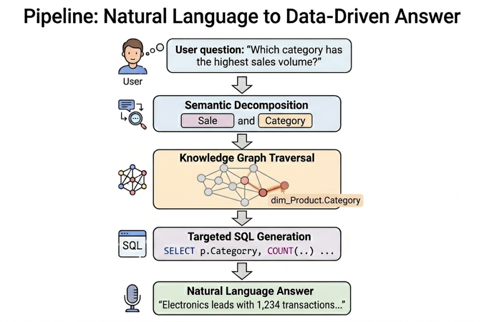
Step 1: Decompose the question. The LLM extracts structured components from the natural language question, applying a decomposition strategy that research has consistently shown to improve SQL accuracy for complex queries:

{
  "intent":   "count_by_category",
  "entities": ["Sale", "Product"],
  "filters":  [],
  "metrics":  ["count"]
}

This structured representation is far more reliable as graph query input than raw natural language. It also separates the “what does the user want?” problem from the “what SQL expresses that?” problem – two very different tasks that traditional NL2SQL conflates into one LLM call.

Step 2: Pull the graph schema: Only mapped concepts (those with :MAPS_TO relationships) are retrieved. Unmapped OWL structural nodes are filtered out automatically, keeping the context focused.
Step 3-4: Generate and execute Cypher:

Synonyms defined in the ontology’s skos:altLabel annotations are resolved at this step -“deals” and “purchases” map to :Sale. So, the Cypher query targets the correct concept nodes regardless of how the user phrased the question.

MATCH (concept:Resource)-[:MAPS_TO]->(t:Table)
WHERE concept.label IN ["Sale", "Product"]
OPTIONAL MATCH (t)-[:HAS_COLUMN]->(c:Column)
RETURN t.name, c.name, c.sql_type, concept.label

The result is a targeted list of tables and columns – the relevant schema slice. This is the Graph RAG advantage in action: graph traversal returns the exact nodes relevant to the question, rather than relying on vector similarity to approximate relevance.

Steps 5-7: SQL generation

• Step 5 loads FK relationships for the identified tables from mapping_output.json, the persisted Phase 1 output. This means the SQL generator arrives with explicit join hints, not guesses.
• Step 6 generates T-SQL. The LLM now sees only the relevant tables, their columns annotated with ontology concept labels, and explicit FK join paths. The prompt for keyword filters is particularly careful: rather than passing a bare value and hoping the model picks the right column, it instructs the LLM to identify which column stores tag/topic values and apply a proper JOIN or subquery. This is the kind of schema-augmented prompting that RAG-based systems have shown to improve accuracy on multi-table joins and nested operations.
• Step 7 executes the SQL against the data warehouse using SQLAlchemy + pyodbc.Here’s an example of what the generated SQL looks like for our running example:

SELECT
    p.Category,
    COUNT(DISTINCT s.SaleID) AS sale_count
FROM [Reporting].[fact_Sales]   s
JOIN [Reporting].[dim_Product]  p  ON s.ProductID = p.ProductID
GROUP BY p.Category
ORDER BY sale_count DESC

Step 8: Answer generation

The final LLM call synthesizes the original question and SQL results into a plain-English answer:

“The category with the highest sales volume is Electronics, with 1,234 recorded transactions, 

nearly 41% more than the next highest category, Apparel (876).”

Why this architecture works

The separation of concerns is the key design win. Here’s how it maps to the challenges the NL2SQL research literature has identified:

Challenge	How this architecture addresses it
Schema complexity	Graph traversal returns only relevant nodes, the SQL generator never sees the full schema
Schema linking accuracy	Mappings are pre-computed, confidence-scored, and human-reviewable, not inferred at query time
Join path inference	FK relationships are explicitly encoded in the graph; LLM receives join hints, not blank slate
Cross-domain generalization	Adding a new domain means updating the graph, not rewriting prompts or fine-tuning models
Ambiguity resolution	The ontology’s rdfs:comment annotations provide semantic grounding that pure schema names lack
Ambiguity resolution	Ontology encodes skos:altLabel synonyms, so that “deals,” “orders,” “purchases” all resolve to the same :Sale class before any SQL is generated

The confidence scoring on mappings (HIGH, MEDIUM, LOW) gives you an operational monitoring signal that standard NL2SQL pipelines entirely lack. After every Phase 1 run, the mapping report surfaces anything that needs human review before queries touch it – a built-in quality gate that catches schema linking errors before they reach production.

How this fits into the broader NL2SQL landscape

It’s worth being explicit about where this approach sits relative to the methods the research community has been exploring.

Most state-of-the-art NL2SQL systems today fall into three categories: in-context learning (zero-shot or few-shot prompting, decomposition, chain-of-thought), fine-tuning (adapting model weights on SQL-specific datasets), and RAG-based systems (dynamic retrieval of schema metadata or example queries). Each has tradeoffs:

• In-context learning is fast to deploy but dependent on prompt engineering and degrades as schema complexity grows.
• Fine-tuning improves domain-specific performance but requires retraining when the schema changes – a significant burden for evolving warehouses.
• RAG-based systems generalize better across domains by retrieving context dynamically, but standard vector-search RAG doesn’t understand relational structure. 

Our approach is a Graph RAG system, the category that research identifies as the current frontier for complex database interactions. By organizing schema elements into a hierarchical structure and pre-indexing relationships, it addresses the specific weakness of flat RAG: the inability to reason about multi-hop relationships between tables. The pre-indexed graph structures also reduce computational overhead during retrieval, since Cypher traversals are far cheaper than running embedding similarity over a full schema at query time.

One important honest caveat: like all RAG-based systems, this approach is slower than a single LLM call. The retrieval steps add latency. For real-time applications this tradeoff needs to be weighed; for analytical queries over a business warehouse, where accuracy matters more than milliseconds, it’s generally the right call.

Technology stack

The pipeline is built on a deliberately minimal stack:

• Neo4j + neosemantics (n10s) for the graph database and OWL import
• Azure OpenAI (GPT-4 family) for all LLM calls, with temperature=0 and JSON mode enforced
• SQL Server as the target data warehouse, accessed via SQLAlchemy + pyodbc
• Python ≥ 3.11, with uv for dependency management and make for workflow commands 

The call_llm(system, user) interface is the only contract between the LLM layer and the rest of the pipeline. Switching to a different provider (Anthropic, Gemini, local models) means changing exactly one file.

What to know before building this

A few practical notes from building and operating this system:

• The ontology is load-bearing. If your ontology has wrong rdfs:domain/ rdfs:range annotations, or missing classes for major fact tables, the Cypher generator will route questions to the wrong tables. The manual review checklist before loading the TTL file isn’t optional, it’s the quality gate for the whole system.
• Mapping confidence is your monitoring signal. LOW confidence mappings after a Phase 1 run are an early warning. They mean the LLM found a weak or ambiguous connection between a concept and a schema object. These need human review before Phase 2 is reliable for questions involving those concepts.
• The graph survives schema changes gracefully. When you add a new table, you add it to combined_schema.json and re-run make build-graph. The mapping step re-runs automatically, and you get a new confidence report for the new additions. You’re not editing prompts or few-shot examples, you’re updating a structured artifact.
• Dynamic schema adaptation remains an open problem. For warehouses where the schema changes very frequently, even the “rebuild the graph” cycle adds overhead. This is an active area of research and future versions of this architecture should explore incremental graph updates rather than full rebuilds on every schema change.
• Phase 2 is partially independent of Neo4j. The FK loader reads from the persisted mapping_output.json rather than querying Neo4j at runtime. This means the graph database only needs to be live during Phase 1 builds and the Cypher execution step, not for every sub-operation in a query.

The bigger picture

Traditional NL2SQL treats the LLM as a schema interpreter. This approach treats it as a reasoning layer on top of a semantic index. The graph does the work of understanding structure and relationships; the LLM does the work of understanding language, generating Cypher, and producing SQL.

The result is a system that scales with schema complexity rather than degrading under it. Adding tables means updating a structured, inspectable, confidence-scored graph, not hoping an increasingly bloated prompt still fits in context and produces correct joins.

The NL2SQL research community has been converging on Graph RAG as the approach that most cleanly addresses the hard parts of this problem: schema linking accuracy, multi-hop reasoning, cross-domain generalization. This pipeline is a concrete implementation of that direction, built for production use on a real enterprise warehouse.

If you’re working with a large data warehouse and finding that off-the-shelf NL2SQL falls apart at the edges, the knowledge graph layer is worth the upfront investment. The Phase 1 build is a one-time cost; the Phase 2 agent benefits from it on every query.