
Deep Learning
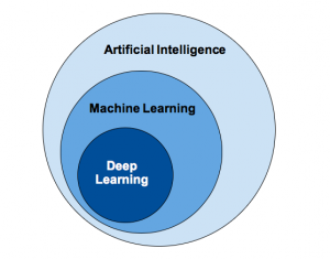
Deep learning is a subset of machine learning, which is a subset of Artificial Intelligence. Artificial Intelligence is a technique that enables a machine to imitate human behavior. Deep learning is a type of machine learning, inspired by the structure of the human brain. This structure is called an artificial neural network.
Deep Learning vs Machine Learning
Machine learning uses algorithms to parse data, learn from that data, and make decisions based on what it has learned. Deep learning structures algorithms in layers to create an “artificial neural network” that can learn and make intelligent decisions on its own. While both fall under the broad category of artificial intelligence, deep learning is what powers the most human-like artificial intelligence.
What is a neural network?
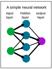
A neural network is a simplification of the human brain. It is made from the layers of neurons. These neurons are the core processing units of the network. One neural network is composed of three types of layers: input, output, and hidden layer. First, we have the input layer, which receives the input and the output layer which predicts the final output. In between, we have the hidden layer, which performs most of the computation required by our network. Also, it is good to mention that neural networks are designed to recognize patterns in the data.
Problem
Let’s try to solve the problem from the previous blog post – Big Data Analyses with Machine Learning and PySpark. In this particular case, we needed to make multiple statistical calculations within a financial institution. One example would be to find if the clients have a deposit or not, based on the number of independent variables. This time we will try to train the model using TensorFlow.
Data preprocessing
Data preprocessing is a crucial step in machine learning and it is very important for the accuracy of the model. This technique allows us to transform the raw data into a clean and usable data set. Using this step, we will make the data more meaningful by rescaling, standardizing, binarizing, and so on. The data set that we are using is preprocessed (more about this, in the previous blog post Data Preprocessing for Machine Learning in Python).
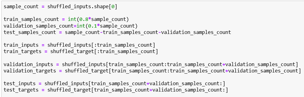
In this case, the only thing that we should do with the dataset is to split it into train, validation, and test sets.
- Training Dataset: The sample of data used to fit the model.
- Validation Dataset: The sample of data used to provide an unbiased evaluation of a model fit on the training dataset while tuning model hyperparameters.
- Test Dataset: The sample of data used to provide an unbiased evaluation of a final model fit on the training dataset.
Also, we will save the data in .npz file format. NPZ is a file format by numpy that provides storage of array data using gzip compression.
TensorFlow
The primary software tool for deep learning is TensorFlow. It is an open-source artificial intelligence library, that uses data flow graphs to build models. TensorFlow is mainly used for Classification, Perception, Understanding, Discovering, Prediction, and Creation. The five main use cases of TensorFlow are:
- Voice / Sound recognition
- Text-based application
- Image recognition
- Time Series
- Video detection
Import the libraries
We need to import the libraries that we are going to use. In our example, we need:
- Numpy – a library for the Python programming language, adding support for large, multi-dimensional arrays and matrices, along with a large collection of high-level mathematical functions to operate on these arrays
- TensorFlow – a free and open-source software library for dataflow and differentiable programming across a range of tasks.
Load the data
First, we need to load the data from the files that we saved before. That can be done by using the load method from Numpy.
Define the model
We need to define the output size – in our case, we are expecting two outputs (1 – yes and 0 – no), so the size will be 2.
Next, we need to define the hidden layer size. The size of the hidden layer should be between the size of the input layer and the size of the output layer. In this case, the hidden layer size will be 30.
The only thing that is left is to define the model. The model in this example is defined using keras. The Sequential model is a linear stack of layers. When we define the model, we need to choose the activation function for the hidden and output layers.
Activation functions
An activation function is one of the building blocks of a Neural Network. If we have a neural network without an activation function, every neuron will perform a linear transformation on the input using only the weights and biases. Defined like this, the neural network will be less powerful and it won’t be able to learn the complex patterns from the data. So, the activation function is used to add the non-linear transformation to the inputs. In the picture below, we can see the common activation functions that can be used.
In this case, we are using ReLU (rectified linear unit) for the hidden layer and Softmax for the output layer.
- ReLU is the most commonly used activation function in neural networks, especially in CNNs. If you are unsure what activation function to use in your network, ReLU is usually a good first choice.
- Softmax is exponential and enlarges differences – push one result closer to 1 while another closer to 0. It turns scores aka logits into probabilities.
Compile the model
In this step, we are configuring the model for training. Compile defines the loss function, the optimizer, and the metrics. We need a compiled model to train (because training uses the loss function and the optimizer).
- Optimizer: Optimization algorithms or strategies are responsible for reducing the losses and providing the most accurate results possible. In this example, we are using an optimization algorithm called Adam. Adam is an optimization algorithm that can be used instead of the classical stochastic gradient descent procedure to update network weights iteratively based on the training data.
- Loss: It’s a method of evaluating how well a specific algorithm models the given data. If predictions deviate too much from actual results, loss function would cough up a very large number. Categorical cross-entropy and sparse categorical cross-entropy have the same loss function – the only difference is that we are using the Categorical cross-entropy when the inputs are one-hot encoded and we are using the sparse categorical cross-entropy when the inputs are integers.
- Metrics: A metric is a function that is used to judge the performance of the model.
Fit the model
When we fit the model, we are actually training the model for a fixed number of epochs (iterations on a dataset). We need to define the Batch size, the maximum epochs, and the early stop.
- Batch size – the number of training examples in one forward/backward pass.
- Maximum epochs – Number of epochs to train the model. An epoch is an iteration over the entire x and y data provided.
- Early stop – Stop training when a monitored quantity has stopped improving. Patience is a number that defines a number of epochs that produced the monitored quantity with no improvement after which the training will be stopped.
Results
In the picture below, we can see the results of the training. If we compare the accuracy (~86%) with the accuracy in the previous blog post (~82%), we can see that in this case, it is larger.
Evaluate the model
Return the loss value and metric values for the model in test mode. In this function, the input data will be our test set. The function will return the scalar test loss (if the model has a single output and no metrics) or a list of scalars (if the model has multiple outputs and/or metrics).

Conclusion
That’s the basic idea of Deep learning. There are many types of deep learning, different kinds of neural networks, variations of architectures, and training algorithms. The idea behind neural networks has been around for a long time, but today it has made great progress. The future of deep learning is particularly bright! The possibilities of deep learning in the future are infinite ranging from driverless cars to robots exploring the universe.