
Introduction
Before we dive into Big Data analyses with Machine Learning and PySpark, we need to define Machine Learning and PySpark.
Let’s start with Machine Learning. When you type Machine Learning on the Google Search Bar, you will find the following definiton: Machine learning is a method of data analysis that automates the analytical model building. If we go deeper into Machine learning and the definitions available online, we can further say that ML is, in fact, a branch of AI that has data as a basis, i.e. all decision-making processes, identifying patterns etc., are made with a minimal human touch. Since ML allows computers to find hidden insights without being explicitly programmed where to look, it is widely used in all domains for doing exactly that – finding hidden information in data.
Machine learning is nothing as it was at the beginning. It has gone through many developments and is becoming more popular day by day. Its lifecycle is defined in two phases: training and testing.
Next is PySpark MLlib which in fact is a machine learning library, which is scalable and works on distributed systems. In PySpark MLlib we can find implementation of multiple machine learning algorithms (Linear Regression, Classification, Clustering and so on…). MLlib comes with its own data structure – including dense vectors, sparse vectors, and local and distributed vectors. The library APIs are very user-friendly and efficient.
Problem
There are many, many challenges that can be solved using these techniques in every industry that we work in. In this particular case, we needed to make multiple statistical calculations within a financial institution. One example would be to find if the clients have a deposit or not, based on the number of independent variables (for ex. age, balance, duration, bank campaign).
How can we solve this problem using machine learning and what will be the final result? To show the solution we’ll use an example of big data that is publicly available on this link.
Solution
Logistic regression is the solution. It is a popular method to predict a categorical response, a special case of Generalized Linear models that predicts the probability of the outcomes.
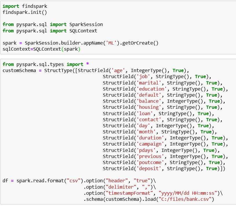
Before we start coding, we need to initialize Spark Session and define the structure of the file. After that, using Spark we can read the data from the csv file. We have a large data set, but in the example, we will use a data set of around 11,000 records.
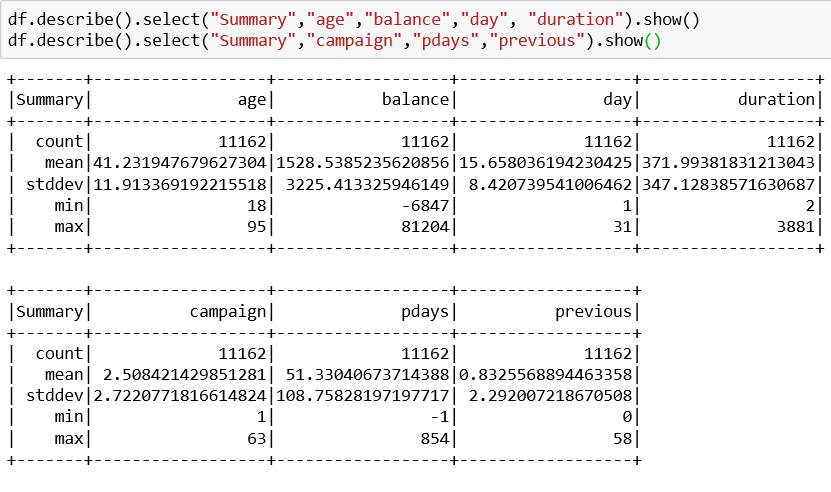
Looking at the tables below, we can see that the minimum value only for one column (previous) is equal to zero (0) and this value is impractical for the example.
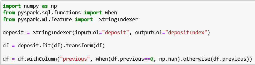
Therefore, we will replace all the zeros with Nan. Also, the field deposit is defined as a string with values ‘yes’ and ‘no’, so we will have to index this field. Using String Indexer, we will change the values from ‘yes’/’no’ to 1/0.
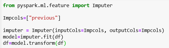
Now, we can simply impute the Nan in the column previous by calling an imputer. The Imputer estimator completes missing values in a dataset, either using the mean or the median of the columns in which the missing values are located. The input columns should be of Double or Float Type.
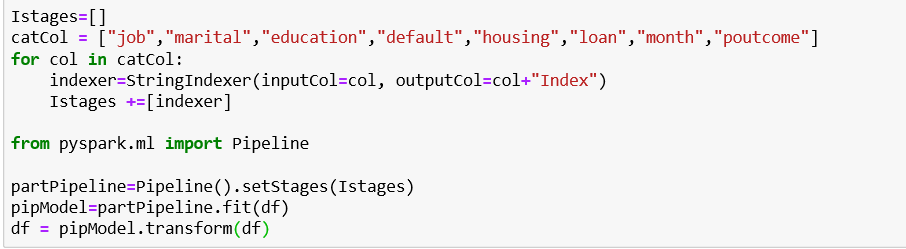
We want to use the categorical fields as well, so we will have to map these fields to a column of binary vectors, mostly with a single one-value. Then, we can find the correlations between the variables and choose which of the variables should we use. Because the categorical fields are of string type, we will use String indexer to encode a string column of labels to a column of label indices.
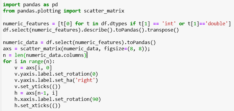
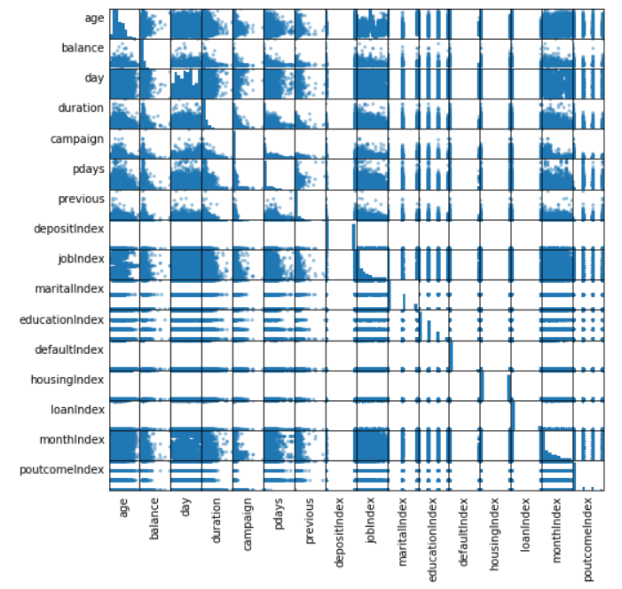
Next, we will find if the numeric features are dependent or not (including the indexed categorical fields). In the picture below, we can see that there aren’t highly correlated numeric variables. Because of that, we will keep all of them for the model. Note: pandas library is used only for plotting – we cannot read a big-data file with pandas, but it is really helpful for plotting.
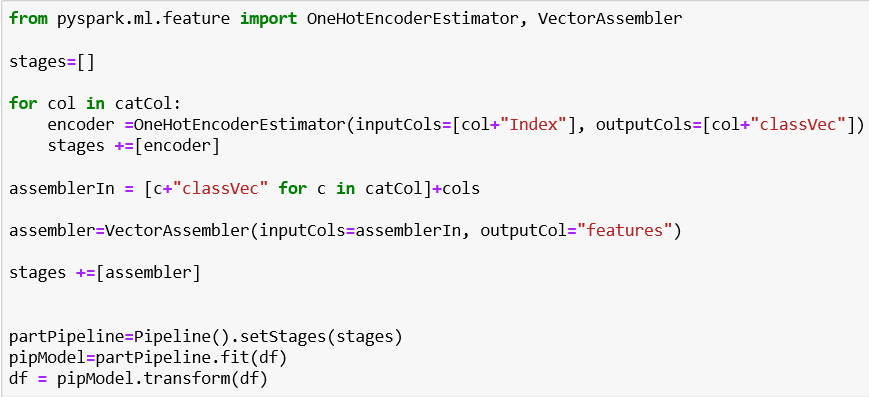
Then, we will use One-hot encoding which maps a categorical feature, represented as a label index, to a binary vector with at most a single one-value indicating the presence of a specific feature value from among the set of all feature values. After this, we will use Vector assembler – it allows us to combine multiple vectors in one and in this case, we will combine the vector with numerical fields with the one with categorical fields that are now transformed. After this, we will use a pipeline. A Pipeline is specified as a sequence of stages, and each stage is either a Transformer or an Estimator. These stages are run in order, and the input DataFrame is transformed as it passes through each stage.
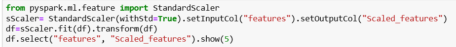
We have created a feature vector and now let’s use StandardScaler to scalarize the newly created “feature” column. StandardScaler is an Estimator that can be fit on a dataset to produce a StandardScalerModel. The model can then transform a Vector column in a dataset to have unit standard deviation and/or zero mean features. In our example, we are using the standard deviation.
After that, we are going to divide the data in a test and train set using the random split method.

Now, let see the percentage of 1 and 0 in our data set.
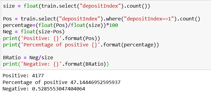
We can see that in our dataset (train) we have 47.14 % positives and 52.85 % negatives. Our tree is balanced so we are good to go.
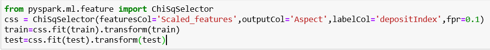
Next, we will use the ChiSqSelector provided by Spark ML for selecting significant features. It operates on labeled data with categorical features. ChiSqSelector uses the Chi-Squared test of independence to decide which features to choose from. We will use the parameter fpr – it chooses all features whose p-values are below a threshold, thus controlling the false positive rate of selection.
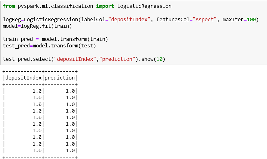
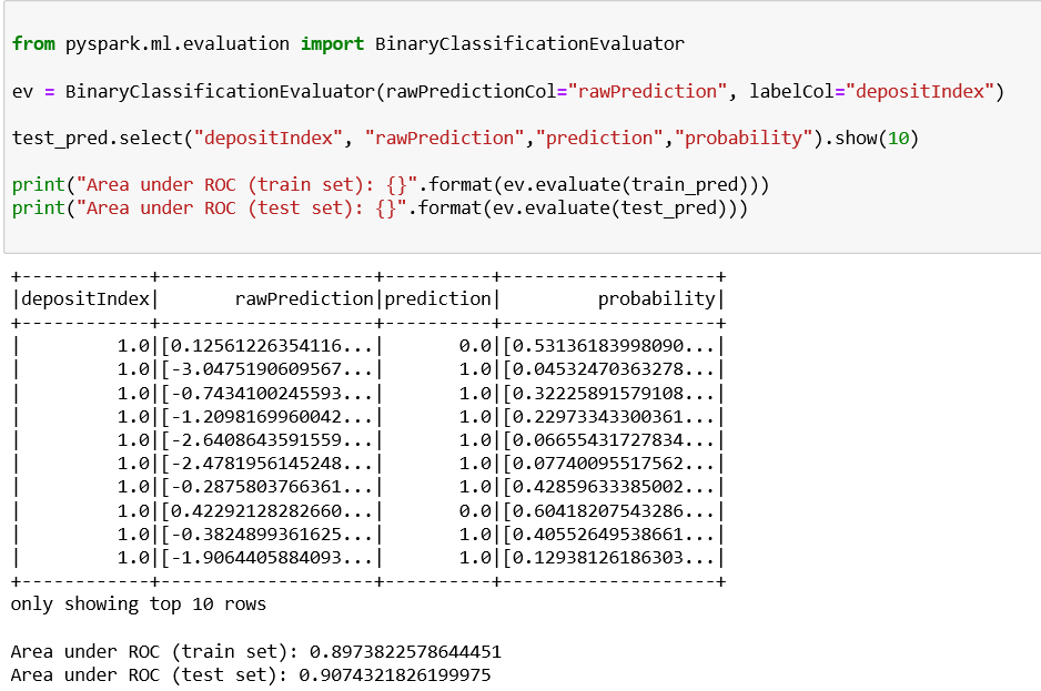
We are going to create the Logistic regression model and we are going to fit the train set. We can see in the final result which of the clients will have a deposit (1) and which won’t have one (0).
Now let us evaluate the model using BinaryClassificationEvaluator class in Spark ML. BinaryClassificationEvaluator by default uses the area under ROC as the performance metric.
Results
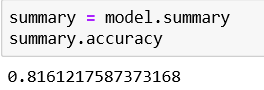
After performing logistic regression on our large dataset, we can conclude the results and determine which clients have a deposit (1) and which don’t (0). We can also see the accuracy of the prediction and in this case, it is approximately 0.82.
The aim of logistic regression is to model the probability of an event that occurs depending on the values of the independent variables. In the future, if we have this kind of problem we can use this approach to make accurate predictions on big data sets.
The Future of Machine learning using big data
Machine learning denotes a step forward in how computers can learn and make predictions. It has applications in various sectors and is being extensively used everywhere. Applying machine learning and analytics more widely lets us respond more quickly to dynamic situations and get greater value from your fast-growing troves of data. Machine learning has been gaining popularity since it came into the picture and it won’t stop any time soon.