
Introduction
In the previous blog post Deep learning using TensorFlow – we saw how we can use TensorFlow on a simple data set. In this example, we are going to use TensorFlow for image classification. The dataset that we are going to use is the MNIST data set which is part of the TensorFlow datasets.
What is image classification?
Image classification refers to a process in computer vision that can classify an image according to its visual content. For example, an image classification algorithm may be designed to tell if an image contains a human figure or not.
Import the libraries
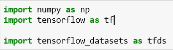
First, we need to import the required libraries. In this example, we need:
- Numpy – a library for the Python programming language, adding support for large, multi-dimensional arrays and matrices, along with a large collection of high-level mathematical functions to operate on these arrays.
- TensorFlow – a free and open-source software library for dataflow and differentiable programming across a range of tasks.
- TensorFlow datasets – a collection of datasets ready to use, with TensorFlow or other Python ML frameworks.
Load and unpack the data
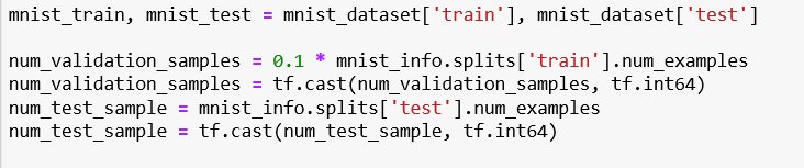
Now, we need to load the data. The MNIST database is composed of 28×28-sized images with handwritten digits.

Also, we need to unpack the data – we are doing this because we need to have the training, validation, and test set.
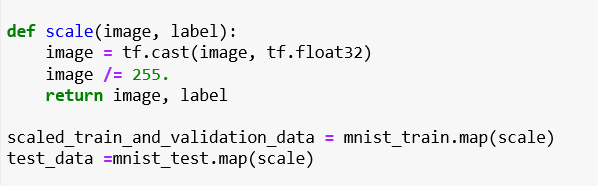
Scale the images
We are going to define a function that will scale the images. We are doing this because the RGB values (Red, Green, Blue) are 8 bits each. The range for each individual color is 0-255 (as 2^8 = 256 possibilities). The combination range is 256*256*256. By dividing it by 255, the 0-255 range can be described with a 0.0-1.0 range where 0.0 means 0 (0x00) and 1.0 means 255 (0xFF).
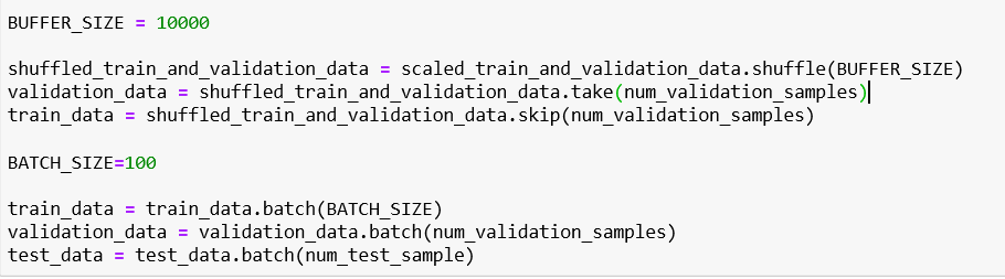
Shuffle the data
Because the data might contain the same values in one part, we need to shuffle it. Buffer size is a scalar that affects the randomness of the transformation. Instead of shuffling the entire dataset, it maintains a buffer of buffer_size elements and randomly selects the next element from that buffer (replacing it with the next input element, if one is available). After shuffling, we need to batch the datasets. The simplest form of batching stacks n consecutive elements of a dataset into a single element is by using the method batch. The Dataset.batch() transformation does exactly this.
Outline the model
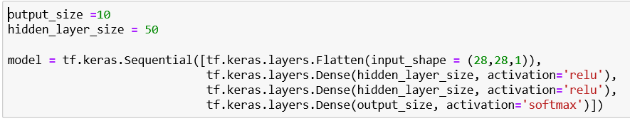
We need to define the output size – in our case, we are expecting outputs from 0-9, so the size will be 10.
Next, we need to define the hidden layer size. The size of the hidden layer should be between the size of the input layer and the size of the output layer. In this case, the hidden layer size will be 50.
The only thing that is left is to define the model. The model in this example is defined using keras. The Sequential model is a linear stack of layers. When we define the model, we need to choose the activation function for the hidden and output layers. If you want to learn more about the activation function, there is a complete explanation in the previous blog post – Deep learning using TensorFlow.
Compile the model
In this step, we are configuring the model for training. Compile defines the loss function, the optimizer, and the metrics. We need a compiled model to train (because training uses the loss function and the optimizer).
- Optimizer: Optimization algorithms or strategies are responsible for reducing the losses and providing the most accurate results possible. In this example, we are using an optimization algorithm called Adam. Adam is an optimization algorithm that can be used instead of the classical stochastic gradient descent procedure to update network weights iteratively based on the training data.
- Loss: It’s a method of evaluating how well a specific algorithm models the given data. If predictions deviate too much from actual results, loss function would cough up a very large number. Categorical cross-entropy and sparse categorical cross-entropy have the same loss function – the only difference is that we are using the Categorical cross-entropy when the inputs are one-hot encoded and we are using the sparse categorical cross-entropy when the inputs are integers.
- Metrics: A metric is a function that is used to judge the performance of the model.

Train the model
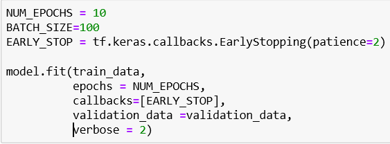
When we fit the model, we are actually training the model for a fixed number of epochs (iterations on a dataset). We need to define the Batch size, the maximum epochs, and the early stop.
- Batch size – the number of training examples in one forward/backward pass
- The number of epochs – Number of epochs to train the model. An epoch is an iteration over the entire x and y data provided.
- Early stop – Stop training when a monitored quantity has stopped improving. Patience is a number that defines a number of epochs that produced the monitored quantity with no improvement after which the training will be stopped.
Results
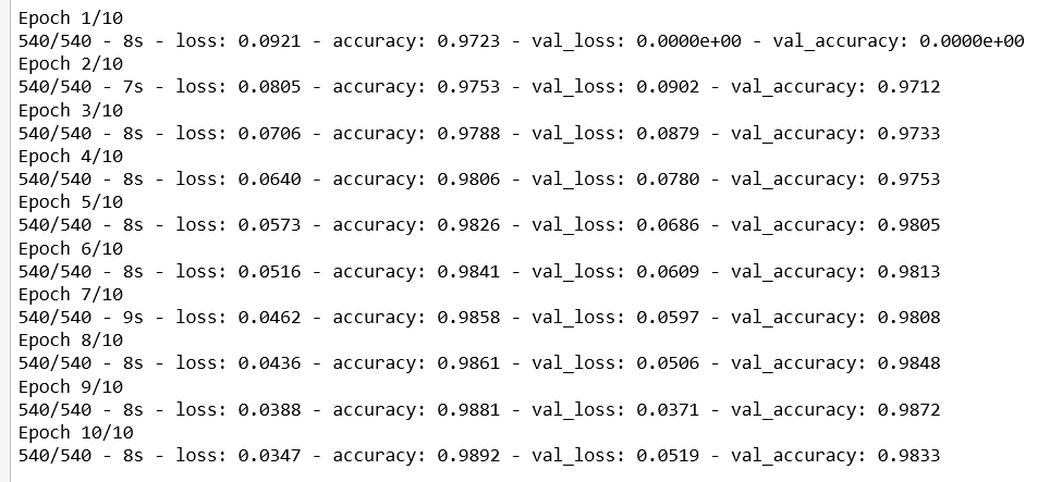
We can monitor the training process by epoch. Every epoch gives us information about the accuracy and the loss using the training and the validation set.
Evaluate the model
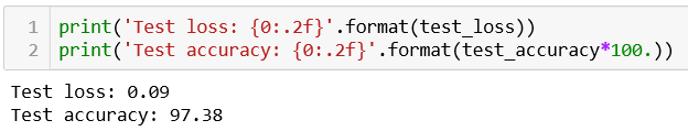
The function returns the loss value and metric values for the model on the test set. In this function, the input data will be our test set. We can print the test loss and the test accuracy – in this example, we have an accuracy of nearly 97%.

Conclusion
This was just a simple example of image classification. There are many more complex modifications we can make to the images. For example, we can apply a variety of filters on the image and the filters use mathematical algorithms to modify the image. Some filters are really easy to use, while others require a great deal of technical knowledge.