

Introduction
Data preprocessing is a crucial step in machine learning for a Data engineer, and it is very important for the accuracy of the model. Data contains noise, missing values, it is incomplete and sometimes it is in an unusable format which cannot be directly used for machine learning models. But what if we use questionable and dirty data? What will the final result be and can the decision be trusted? Preprocessing data is the key – the goal with the preprocessing is to get more meaningful data that can be trusted.
These techniques allow us to transform the raw data into a clean and usable data set and make the data more meaningful by rescaling, standardizing, binarizing and so on.
Data Preprocessing Concepts
In the example below, we will use one file that contains cars and it can be downloaded from https://www.kaggle.com/antfarol/car-sale-advertisements. We will use Python for data preprocessing. We’ll use several libraries of importance:
- Pandas – a package providing fast, flexible and expressive data structures designed to make working with “relational” or “labeled” data both easy and intuitive;
- scikit-learn – a library that provides many unsupervised and supervised learning algorithms and is built upon NumPy, pandas, and Matplotlib;
- Statsmodel – a package that allows users to explore data, estimate statistical models and perform statistical tests;
- Matplotlib – a plotting library;
- Seaborn – a library for making statistical graphics in Python. It is built on top of matplotlib and closely integrated with pandas data structures.
There are a lot of methodologies and concepts that can be used, but in this example, we will only see some of them:
- Handling missing values
- Dealing with outliers
- Multicollinearity
- Dealing with categorical values
- Standardization
Load the Data
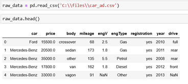
The first step is loading the data. We can read the .csv file and using the method head we can see the first 5 rows in our data set.
Discovering the Data
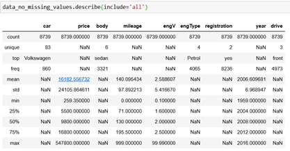
Now, let’s discover the data. We can use the describe method – if we use this method we will get only the descriptive statistics of the numerical features. We can include all of them by using include=’all’.
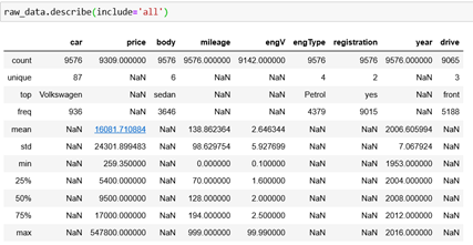
We can see the unique values and the most common category for every column. For example, we can see that the column registration contains 9015 values of yes and that it has two unique values. Also, we can see the mean, standard deviation, maximum and minimum values and so on.
Handling Missing Values
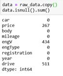
An easy way to check for missing values is to use the method isnull. We will get a data frame with true (1) and false (0) values, so we will sum the values and we can see in which column we have missing values.
We can handle the missing values in two ways:
1. Eliminate missing values:
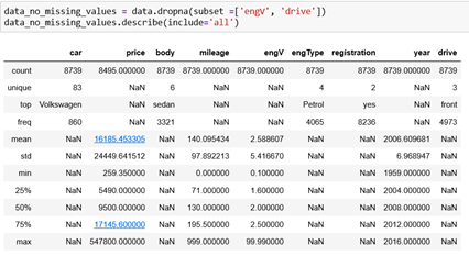
a. Eliminate rows: we can remove the rows with unacceptable missing values. This can be done by using the method dropna. This way, we will exclude the rows that contain missing values.
b. Eliminate columns: If the column has 95% or more missing values, it can and needs to be deleted because the estimation of the missing values cannot be trusted as it will be calculated from the 5% (or less) of the data, hence, it is irrelevant.
2. Estimate missing values: if the only acceptable percentage of values is missing, we can estimate the values. This can be done by filling the values in with the mean, median or most frequent value of the respective feature.
Also, there are multiple methods that can be used for imputing the missing values. We can use Simple imputer, Iterative imputer or Categorical Imputer. Categorical imputer is used for imputing the categorical features.
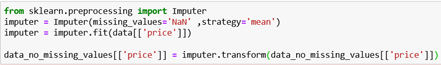
After this, if we call the method describe we can see that in the column price we have the same count as car and body. Our missing values are replaced with the mean of all values in this column.
Dealing with Outliers
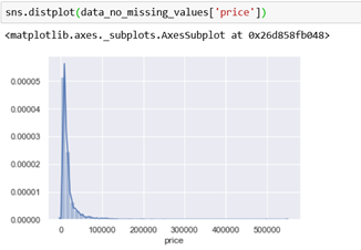
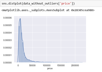
If we are working with regression, this is a very important topic. We will plot the distribution for the column price. For an optimal result, we are looking for a normal distribution. But, the price has an exponential one. This will be a problem if we are using regression. We can see in the table above, that the minimum value for the price is 259, the maximum is 547,800 and the mean value is 16,182. Also, we can see that 25% of the values are under 5,500 and 75% are under 16,800. So, in this case, we have outliers. Outliers are observations that lie on abnormal distance from other observations in the data and they will affect the regression dramatically. Because of this, the regression will try to place the line closer to these values.
The common rule is to remove everything that is 3 * standard deviations far from the mean. What does this mean? For normally distributed values there is a known rule: 68-95-99.7. The rule can be explained as:
- 68% of the data is distributed in the interval [mean – standard deviation, mean + standard deviation],
- 95% of the data is distributed in the interval [mean – 2 * standard deviation, mean + 2 * standard deviation],
- 99.7% of the data is distributed in the interval [mean – 3 * standard deviation, mean + 3 * standard deviation].
Based on this, we can say that the values that are out of the interval [mean – 3*std, mean + 3*std] are outliers and these values can be removed.
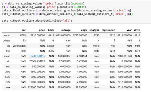
The maximum value is still far away from the mean, but it is acceptably closer. We can now plot the distribution and we can see that the data is still distributed the same way, but with fewer outliers. We can do this with the column mileage as well.
Multicollinearity
Multicollinearity exists whenever an independent variable is highly correlated with one or more of the other independent variables in a multiple regression equation. Multicollinearity is a problem because it undermines the statistical significance of an independent variable.
Unfortunately, using scikit-learn we cannot straight forward determine if multicollinearity exists. We can do this by using statsmodels. One of the best ways to check for multicollinearity is through VIF (variance inflation factor). VIF produces a measure that estimates the degree to which the square root of the standard error of an estimate is bigger, compared to a situation when the variable was completely uncorrelated with the other predictors. The numerical value for VIF tells us (in decimal form) the percentage the variance (i.e. the standard error squared) is inflated for each coefficient. For example, a VIF of 1.9 tells us that the variance of a particular coefficient is 90% bigger than what we would expect if there was no multicollinearity — if there was no correlation with other predictors.
In our example, we can say: if mileage is smaller – the price will be bigger. Also, if the car is older, the price will be smaller. So, we can check for multicollinearity for these three columns.
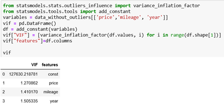
When VIF value is equal to 1, there is no multicollinearity at all. Values between 1 and 5 are considered perfectly okay. But, there is no precise definition of what values would be acceptable. We can find in different resources that values below 5, 6 or even 10 are acceptable. So, in our example, we can see that all of the values are below 5 and they are okay. We can rarely find data where all the features have value below 5. We can say that our data set doesn’t have multicollinearity. If we had multicollinearity we should drop the column using the method drop. As input we will set the column that we want to be removed and axis = 1 – this means that we will delete a column. For example, let’s say that we want to delete the column year from our dataset.

Dealing with Categorical Values
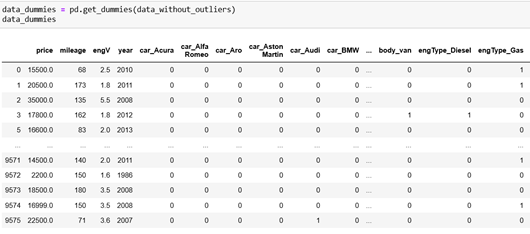
Dummy coding is a commonly used method for converting a categorical input variable into a continuous variable. ‘Dummy’, as the name suggests, is a duplicate variable that represents one level of a categorical variable. The presence of a level is represented by 1 and absence is represented by 0. For every level present, one dummy variable will be created. In Python, we can use the method get_dummies which returns a new data frame that contains one-hot-encoded columns.
Standardization
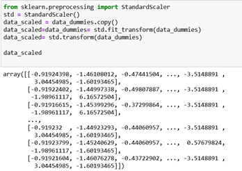
After dealing with categorical values, we can standardize the values. They are not on the same scale; therefore, our model will give more weightage to the ones that have bigger values which is not the ideal scenario as the other columns are important for building the model. In order to avoid this issue, we can perform standardization.
Note: In some examples, the standardization might not give better results – they can be even worse.
We will use the class StandardScaler from scikit-learn. The idea behind StandardScaler is that it will transform the data such that its distribution will have a mean value 0 and a standard deviation of 1.
Date and Time Transformation
Although there are no date or time columns in our database, we can often find variables that denote dates or time. Thus, it is important to know how we can work with such variables when defining a machine learning model. Also, we need to know how we can preprocess the date/time fields before using them in any machine learning model. We need to extract the features from the date/time type that are going to be very useful for building our model. For example, from a date variable, we can extract basic features like:
- Month, day, year, quarter and day of the week
- Semester
- Weekend or not
Extract Basic Features
For extracting the features, we will use Pandas.Series.dt. It can be used to access the values of the series as datetime and return several properties.
We need to convert the column in datetime type. Now we can work with this column because it has the appropriate type.
Extract Month, Day, Year, Quarter and Day of Week
We can get month, day, year, quarter, and day of the week from the datetime object easily.
Extracting Semester
This is more specific as we need to do some calculations to achieve this. We will use the function isin to check whether values are contained in Series. The function returns a boolean Series showing whether each element in the Series matches an element in the past sequence of values exactly.
Extracting Information about Weekend
We will use the same function isin and if the day is Saturday or Sunday, we will add 1 – otherwise 0.
Conclusion
The aim of this article is to show how some of the data preprocessing techniques can be used and gain a deeper understanding of the situations where those techniques can be applied. There are other forms of data cleaning that are useful as well, but for now, we are covering those that are important before the formulation of any model. Better and cleaner data outperforms the best algorithms, so it’s beneficial to master your data. If we use a very simple algorithm on data that is cleaned, we will get very impressive and accurate results.
If you are interested in this topic, do not hesitate to contact us.