
Overview
Application Performance Monitoring (APM) is one of the most important aspects of the IT industry. Monitoring ensures that applications, servers, networks, etc. work as expected. In addition, it identifies/resolves issues very fast before users even know that there is a problem in the system.
Problem
One of the common problems with every environment/system/application is to identify node performance degradation. The usual suspects for this are CPU, memory, and disk. This is not a trivial task where you have many active Nodes in different environments and you want to make a data comparison. We use PRTG as a monitoring tool in our current environments, but the tool’s native dashboards are more or less fixed and not very customizable.
Case
We have chosen a cloud environment with all of its rich features and services, i.e. an environment that will match our needs for a robust and customizable solution. In our specific case, we will review and explain the process of performance logs monitoring on on-premise Virtual Machines (VM) that are connected to the Microsoft Azure cloud computing service. In particular, we will show you how to generate consolidated CPU/Memory reports for several nodes in one or more environments.
The solution provides:
- Centralized node monitoring
- Power BI reports and visualizations
- A good overview of usage/free – CPU/Memory in a certain time frame.
Solution
The solution relies on two log queries: one for Memory and one for CPU monitoring. Each query runs for every virtual machine separately and collects data from the Logs within the Log Analytics workspace. Using functions/methods/variables from the performance pane (Perf), you cannot select more machines in one query and render a time chart with multicolor spikes.
// Virtual Machine’s available memory
// Chart the VM's available memory over the last 30 days.
Perf
| where TimeGenerated > ago(30d)
| where ObjectName == "Memory" and
(CounterName == "Available MBytes Memory" or // the name used in Linux records
CounterName == "Available MBytes") // the name used in Windows records
| project TimeGenerated, CounterName, CounterValue
| render timechart
// Chart CPU usage trends
// Calculate CPU usage patterns over the last 30 days, chart by percentiles.
Perf
| where TimeGenerated > ago(30d)
| where CounterName == "% Processor Time"
| where ObjectName == "Processor"
| summarize avg(CounterValue) by bin(TimeGenerated, 30min) // bin is used to set the time grain to 30 minutes
| render timechart
// Perf table stores performance counters for Windows and Linux computers
// Counters are specified using ObjectName (performance object), InstanceName and CounterName
// % Processor Time captures CPU activity, ObjectNames can be Processor, Process and Process Information
Finally, we export the Perf queries for every selected machine as Power BI M queries. Azure endpoints are included in the exported queries.
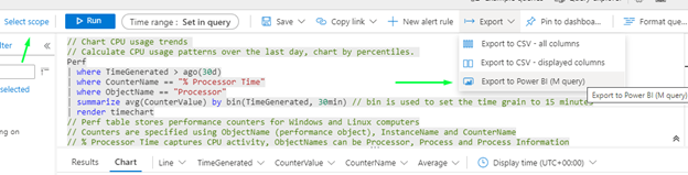
Below are two samples of the exported queries:
- Memory:
let AnalyticsQuery =
let Source = Json.Document(Web.Contents("https://api.loganalytics.io/v1/subscriptions/<subscriptions account number>/resourceGroups/Group-VM/providers/Microsoft.Compute/virtualMachines/Node01/query",
[Query=[#"query"="
Perf
| where TimeGenerated > ago(30d)
| where ObjectName == ""Memory"" and
(CounterName == ""Available MBytes Memory"" or
CounterName == ""Available MBytes"")
| project TimeGenerated, CounterName, CounterValue
| render timechart
",#"x-ms-app"="AzureFirstPBI",#"scope"="hierarchy",#"prefer"="ai.response-thinning=true"],Timeout=#duration(0,0,4,0)])),
TypeMap = #table(
{ "AnalyticsTypes", "Type" },
{
{ "string",   Text.Type },
{ "int",      Int32.Type },
{ "long",     Int64.Type },
{ "real",     Double.Type },
{ "timespan", Duration.Type },
{ "datetime", DateTimeZone.Type },
{ "bool",     Logical.Type },
{ "guid",     Text.Type },
{ "dynamic",  Text.Type }
}),
DataTable = Source[tables]{0},
Columns = Table.FromRecords(DataTable[columns]),
ColumnsWithType = Table.Join(Columns, {"type"}, TypeMap , {"AnalyticsTypes"}),
Rows = Table.FromRows(DataTable[rows], Columns[name]),
Table = Table.TransformColumnTypes(Rows, Table.ToList(ColumnsWithType, (c) => { c{0}, c{3}}))
in
Table
in AnalyticsQuery
- CPU
let AnalyticsQuery =
let Source = Json.Document(Web.Contents("https://api.loganalytics.io/v1/subscriptions/<subscriptions account number>/resourceGroups/Group-Snaplogic/providers/Microsoft.Compute/virtualMachines/Node01/query",
[Query=[#"query"="
Perf
| where TimeGenerated > ago(30d)
| where CounterName == ""% Processor Time""
| where ObjectName == ""Processor""
| summarize avg(CounterValue) by bin(TimeGenerated, 30min)
| render timechart
",#"x-ms-app"="AzureFirstPBI",#"scope"="hierarchy",#"prefer"="ai.response-thinning=true"],Timeout=#duration(0,0,4,0)])),
TypeMap = #table(
{ "AnalyticsTypes", "Type" },
{
{ "string",   Text.Type },
{ "int",      Int32.Type },
{ "long",     Int64.Type },
{ "real",     Double.Type },
{ "timespan", Duration.Type },
{ "datetime", DateTimeZone.Type },
{ "bool",     Logical.Type },
{ "guid",     Text.Type },
{ "dynamic",  Text.Type }
}),
DataTable = Source[tables]{0},
Columns = Table.FromRecords(DataTable[columns]),
ColumnsWithType = Table.Join(Columns, {"type"}, TypeMap , {"AnalyticsTypes"}),
Rows = Table.FromRows(DataTable[rows], Columns[name]),
Table = Table.TransformColumnTypes(Rows, Table.ToList(ColumnsWithType, (c) => { c{0}, c{3}}))
in
Table
in AnalyticsQuery
The exported Power Query Formula Language (M Language) can be used with Power Query in Excel and Power BI Desktop.
For Power BI Desktop follow the instructions below:
- Download Power BI Desktop from https://powerbi.microsoft.com/desktop/
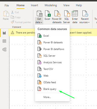
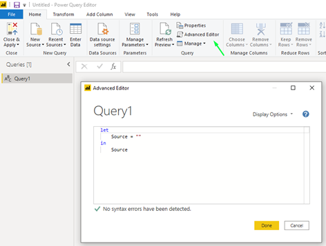
- In Power BI Desktop select: ‘Get Data’ -> ‘Blank Query’->’Advanced Query Editor’
- Paste the M Language script into the Advanced Query Editor and select ‘Done’
Then we import every query as a blank query,
Note: Once you complete the imports you will need to assign some data source credentials in order for the data to be accessed from Azure Logs through your account. Power Query caches your credential information so you only have to enter it once. However, Personal Access Tokens expire and you may need to update or change your authentication information.
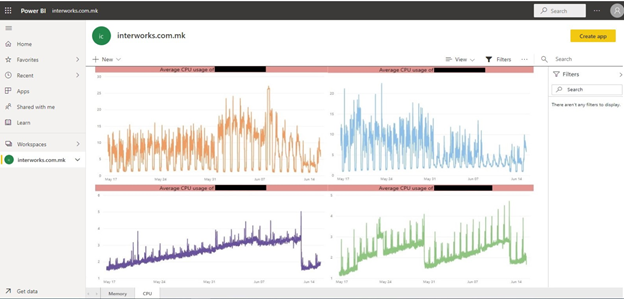
After the queries have been added you can visualize your data through ‘Visualizations’.
For this example, we have the data to be visualized from the CounterValue (average of the values collected) and TimeGenerated:
* The maximum number of data points density for Power BI visuals is 30,000.
From the View tab, a Mobile Layout can be created.
Next you publish your .pbix file to one of your workspaces.
This report can be shareable within your organization, refreshed on a scheduled time basis, re-edited, etc.
Conclusion:
How you use Power BI is based on the feature or service of Power BI that best suits your situation. From the example above with Power BI we can achieve stable environments as with every other deployment we can monitor spikes of CPU/Memory usage. This way problems such as memory leakage or high CPU consumption can be detected on time and appropriate measures can be taken over. Also, this could be useful when performance testing is done on a project/application so we can monitor how much load the system can take without any issues arising.
With all of this we can achieve:
- Lower costs for node resources needed
- Easier comparison between node usage
- Maximum use of available resources
- Better data comparison
- Enhanced personalized and shareable reports
- Transparency and accountability