
We know that humans learn from their past experiences and machines follow instructions given by humans. What if humans can train machines to learn from past data and do what humans can do much faster? And this is possible with Machine Learning. Machine Learning is a field in technology that allows machines to learn from data and self-improve. It is been around for a long time, but it’s becoming increasingly useful and relevant for three reasons:
- There is more data than ever before.
- Computers are more powerful than they used to be.
- There are better machine learning algorithms.
As a result, machine learning is already present all around us. For example, it is used to recommend purchases on the Internet or to detect fraud on a credit card.
Azure Machine Learning Studio (Classic)
Machine Learning Studio (classic) is a tool that can be used to build, test, and deploy machine learning models. Studio (classic) publishes models as web services and they can easily be consumed by custom apps or BI tools. It can be used by data scientists and data engineers to complete their machine learning tasks end-to-end in a productive way. [Source: Microsoft]
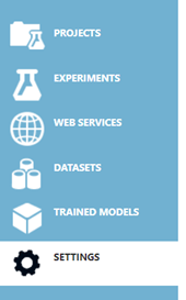
Here are the main features of the Azure Machine Learning Studio:
- Projects – a place where we can create the Machine learning experiments and datasets all into one. We can create multiple experiments and use multiple datasets and they can belong to one project.
- Experiments – the place where we actually create the models using the UI interface. We can use some sample datasets or upload our dataset.
- Web services and trained models – the place where we publish the trained model.
- Datasets – the place where we upload the datasets that we are going to use in building our machine-learning model.
In our blog post, we focus on predicting the temperature based on numerous features that are available in the dataset. The dataset is composed of multiple features like summary, temperature, apparent temperature, humidity, wind speed, wind bearing, visibility, pressure, etc. Based on some of these features, we will try to predict the temperature.
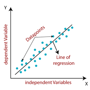
Linear regression
Linear Regression is a supervised machine learning algorithm where the predicted output is continuous and has a constant slope. It’s used to predict values within a continuous range, (e.g. sales, price) rather than trying to classify them into categories (e.g. cat, dog). Here is the visual representation of linear regression:
Solution
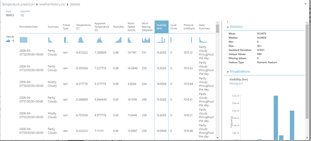
The first step is getting the dataset that we are going to use. We will use the dataset called weather history which contains information about the hourly/daily temperature summary for Szeged, the Hungary area, between 2006 and 2016. We will upload the dataset and then we can find this dataset in saved datasets -> My datasets.
If we want to see the data and the statistics about the features like mean, most frequent value, and so on, we can do that with the Visualize option:
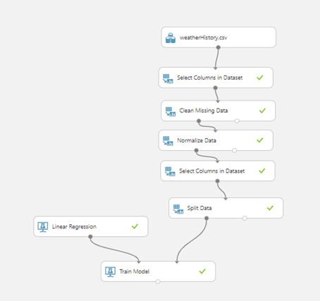
The next step is selecting the columns that we are going to use. To do this, we will use the module Select columns in the dataset. In our example, we are using all columns.
After this, we need to clean the missing data. We will use the module Clean missing data. We are going to use the option Replace using MICE (multiple imputations by chained equations). Basically, missing data is predicted by observed data, using a sequential algorithm that is allowed to proceed to convergence. It starts by filling in the missing data with plausible guesses at what the values might be. For each variable, predict the missing values by modeling the observed values as a function of the other variables. At each step, it updates the predictions of the missing values.
After the data is cleaned, we will normalize the dataset by using the module Normalize Data. Normalization is a technique often applied as part of data preparation for machine learning. The goal of normalization is to change the values of numeric columns in the dataset to use a common scale, without distorting differences in the ranges of values or losing information. Normalization is also required for some algorithms to model the data correctly.
In our example, we will use the z-score. The mean and the standard deviation are computed for each column separately. This is the formula that is used for calculating the Z-score, the population mean, and population standard deviation.
Now, we have to select the columns that we are going to use in our prediction. Why do we do this again? Because we need to select the columns that are important for our prediction. What does important mean? This time, we need to include only the columns that we think are important for our prediction and that will influence the temperature. This is something that we can play around with – we can try with different features. In our example, we are using the apparent temperature, humidity, wind speed, wind bearing, and temperature.
The next step is splitting the dataset into training and testing. In this example, we will use 80% of the data for training and 20% for testing. After this, we can choose our model – and in our example, because we are predicting the temperature we are solving a regression problem. We are going to use the Linear regression module. We will use the module Train model for training the model. Here we need to specify the column that we are trying to predict, ie the temperature. This can be done by launching the column selector and choosing the appropriate column. Now we can see that our diagram looks like in the picture below:
After this, we can see how our model performs by using the module Score model. We need to use the test data for this model – so we are going to connect this module to the Train model and split data – the right part of this module which contains the testing dataset. The last step is evaluating the model and to achieve it, we are going to use the module Evaluate model and we will connect this module to the Score model. Now, we can see how the diagram looks like:
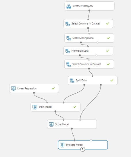
Let’s try to run the experiment and see how our model performs. When we run the experiment, it will execute step by step and actually will run each module one at a time. Once it finishes, we can see green checkmarks beside every module, which means that they have run successfully.
Following is a picture of how our model performed on the test set:
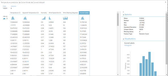
The last column Scored Labels is actually the predicted value and temperature is the actual temperature. We can see that some of the values are pretty close, while some of them are not. So, we can try to improve the model by using some other features or using additional data transformations.
We can see the evaluation of our model as well as the accuracy:
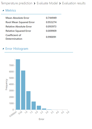
The meaning of the metrics is:
- Mean absolute error (MAE) measures how close the predictions are to the actual outcomes – a lower score is better.
- Root mean squared error (RMSE) creates a single value that summarizes the error in the model. By squaring the difference, the metric disregards the difference between over-prediction and under-prediction.
- Relative absolute error (RAE) is the relative absolute difference between expected and actual values; relative because the mean difference is divided by the arithmetic mean.
- Relative squared error (RSE) similarly normalizes the total squared error of the predicted values by dividing the total squared error of the actual values.
The last step is publishing the experiment – we can create a model that will be public or only available with a direct link.
Conclusion
This is a simple example of how we can use the Azure Machine Learning Studio (classic) to build a simple Linear Regression model. We can build more complex models and also, we can use different machine learning algorithms based on the requests that we have.
With Microsoft Azure ML studio, it’s very easy to start developing and testing machine learning models. And regardless of the development environment you like, I encourage you to explore machine learning and find your inner data scientist?
If you want to discuss Azure Machine Learning Studio and how you can use it in your projects or other Azure DevOps advantages, feel free to contact us.