
Why Big Data?
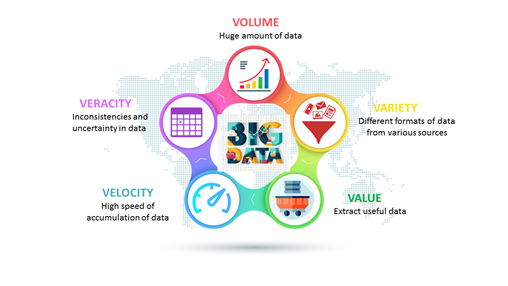
We all use smart devices, but have you ever wondered how much data it generates in the form of items like texts, images, emails, phone calls, photos, searches, and music? Approximately 40 exabytes of data are generated every month by a single smartphone user. Now if we multiply this number with 50 billion users, that is a lot for our minds to process. This amount of data is quite a lot for a traditional computing system to handle and this massive amount of data is what we say big data. If we want to classify some data as big data, it needs to satisfy the concept of 5Vs, as shown in the picture below.
Big data algorithms
Organizations gather and store a lot of data and we no longer doubt the value of this process. Now, organizations are heavily focused on using methods or algorithms that might extract the most valuable and most important information that the data represents. So, to achieve this we should find a process that will make sense of the data – find what is valid, relevant, and usable and how to use it. The more data there is, the more difficult it is to process, store, and analyze it. But, let’s see this from a different perspective – the more data the organization has – the more accurate the predictions are. We need to find a way to make sense of a huge amount of data – this means making use of statistical models to create algorithms to sort, classify, and process big data.
Faced with this problem, we decided to suggest some important and valuable algorithms for big data that can solve multiple problems. We will describe the following algorithms:
- Linear Regression
- Classification using Ada Boost Classifier
- K-nearest neighbor
- K-means clustering
Use-case for Linear Regression
Linear regression is one of the most commonly used and is one of the basic algorithms. The data can be easily visualized along with the way the input and output data are correlated.
When using linear regression, we have two sets of variables – the first one is the predictor (independent) variable and the other one is the response (dependent) variable. As a result of the linear regression, we are expecting a relationship in the form of a formula that explains the dependent variable in terms of the independent one. Once the relationship is obtained, the dependent variable can be predicted for any instance of the independent variable.
Making predictions using Linear Regression
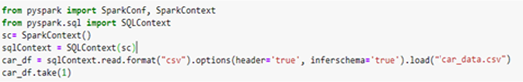
As we mentioned above, this algorithm is mostly used for predicting the values of some variables based on other variables that are in the same dataset. In the following example, we will use a dataset that contains data for various cars that are on sale. Based on the provided information, the goal is to come up with a model to predict the selling price.
We will build a linear regression model using Python, Spark, and MLlib so that we can have an intuition for machine learning when it comes to working with big data.
First, we initialize the Spark Context and load the data from the CSV file:
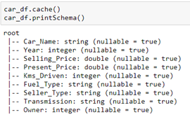
In the picture below, we can see the schema for car_df in a tree format:
We can obtain descriptive analytics and analyze the data from the data set. In this case, we will use the Pandas library just for better representation of the data. We wouldn’t use Pandas when working with big data, but if we want to see the descriptive statistics in a better form, we can use it just for a preview:
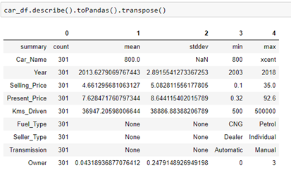
This data set contains categorical and numerical values. We want to use categorical fields as well, so we will need to map these to a column of binary vectors. After this step, we can perform the correlations between variables and choose which to use. We can see that the categorical variables are of type string, so we will use String Indexer to encode a string column of labels to a column of label indices.

Now we are ready to find a correlation between independent variables and target variables. The correlation coefficient range is between -1 and 1. When the number is closer to 1, we can say that we have a strong positive correlation, which means if the value of the independent variable goes up the value of the dependent variable also goes up. When the coefficient is closer to -1 we can say that there is a strong negative correlation, which means if the value of the independent variable goes up, the value of the dependent variable goes down. Coefficients close to zero mean that there is no linear correlation.

From the results above, we can see that there isn’t a strong correlation between the Selling price and Kms Driven and between the Selling price and Owner. So, we won’t use these two columns. We will build the model using the other columns.
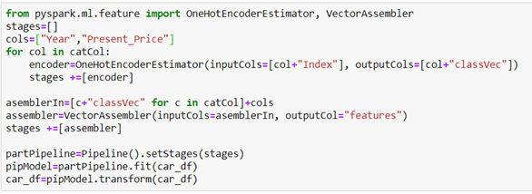
One-hot encoding is a process by which categorical variables are converted into a form that could be provided to ML algorithms for better prediction. It will create a duplicate variable that represents one level of a categorical variable. The presence of a level is represented by 1 and absence is represented by 0. We will use this method to map categorical features that are already transformed as a label index, to a binary vector. Vector assembler is used to combine multiple vectors in one, so we will use it to combine vectors with a numerical and categorical feature that are already transformed.
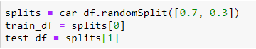
The next step is splitting the already prepared data between the train set (70%) and test (30%) set. The training set is used for training the ML model and the testing set is for testing the obtained model.
Now, let’s create an instance of the Linear Regression model using the columns feature and Selling_Price and also instantiate a prediction named column for our predictions.

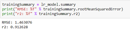
The code below shows metrics for the summarized model over the training set. RMSE shows the difference between predicted and actual values of the car’s Selling price. R squared in our case indicates that in our model, approximately 91% of the variability in “Selling_Price” can be explained using the model.
We must be cautious, because not always a good approximation of the training set, will be good on the test set. So, we will see the R squared on the test set.
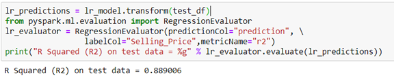
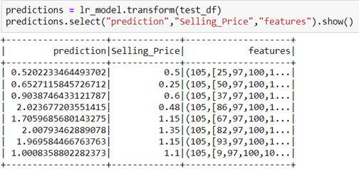
In our case, it is lower, but still acceptable. Finally, we can see the predicted values from our model:
Classification using Ada-Boost Classifier
Boosting algorithms gained a lot of popularity in data science and machine learning in the last few years. They are used to achieve high accuracy for predictions in multiple areas, such as business, government, health, sales, and so on. Boosting algorithms combine multiple low-accuracy models to create a high-accuracy model. Some of the boosting algorithms that are widely used in machine learning are Ada-Boost, Gradient Boosting, and XGBoost.
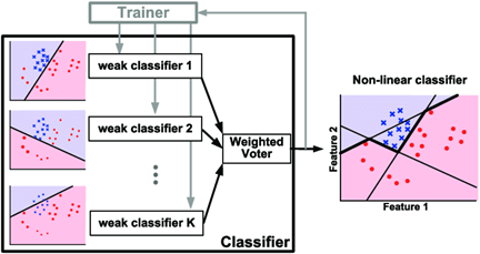
Ada-boost or Adaptive Boosting is one of the boosting algorithms that combine multiple classifiers to increase the accuracy of classifiers and it is defined as an iterative ensemble method. The basic concept behind Ada-boost is to set the weights of classifiers and train the data sample in each iteration such that it ensures accurate predictions of unusual observations.
Ada-boost should meet two conditions:
- The classifier should be trained interactively on various weighted training examples.
- In each iteration, it tries to provide an excellent fit for these examples by minimizing training errors.
How does Ada-boost work? First, Ada-boost selects a training subset randomly. It iteratively trains the AdaBoost machine learning model by selecting the training set based on the accurate prediction of the last training and it assigns the higher weight to wrong classified observations so that in the next iteration these observations will get a high probability for classification. The next step is assigning the weight to the trained classifier in each iteration according to the accuracy of the classifier. Those classifiers that are more accurate, will get higher weight. This process iterates until the complete training data fits without any error or until it reaches the specified maximum number of estimators.
In Python, we can use the algorithm from scikit-learn. In the example, we will try to classify the flowers that are contained in the iris dataset.

Now, we will load the dataset in a variable and we will get the inputs and the target in different variables.

We will use the method train_test_split to split the dataset into training and test set. The data set will be split in a way that 80% of the data will be for training and 20% for testing.

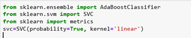
Now, we will use C-Support Vector Classification. SVC implements the “one-versus-one” approach for multi-class classification. In total, n_classes * (n_classes – 1) / 2 classifiers are constructed and each one trains data from two classes. To provide a consistent interface with other classifiers, the decision_function_shape option allows us to monotonically transform the results of the “one-versus-one” classifiers to a “one-vs-rest” decision function of shape (n_samples, n_classes). The input parameters are:
- Probability – If we want to enable probability estimates.
- Kernel – Specifies the kernel type that will be used in the algorithm. It must be one of the following: linear, poly, rbf, sigmoid, precomputed, or callable.
Now, we will create Ada-boost Classifier with n_estimators equal to 50, base_estimator equal to svc, and learning_rate equal to 1.
- N estimators – the maximum number of estimators at which boosting is terminated.
- Base estimator – the base estimator from which the boosted ensemble is built.
- Learning rate – shrinks the contribution of each classifier by learning_rate.

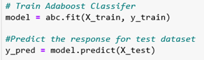
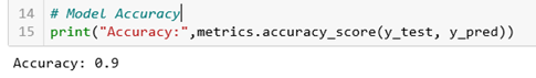
The last step includes training and testing the model using the training and test set accordingly.
We can see that we have an accuracy of 90% on our test set, which is very high and acceptable.
K-nearest neighbor
K-nearest neighbor, known as “lazy learner” because the training phase is very limited, is a classification algorithm as well. In the learning process, the training set is needed. As new instances are evaluated, the distance to each data point in the training set is evaluated and there is a consensus decision as to which category the new instance of data falls into based on its proximity to the training instances.
K-nearest neighbors might be computationally expensive and it depends on the training set (its scope and size), but it is often chosen because it is easy to use, easy to train, and easy to interpret the results. It is often used in search applications when you are trying to find similar items.

So, we can implement this algorithm in Python. The first step is composed of a calculation of Euclidean distance between two vectors. The Euclidean distance between two vectors is the length of the line segment that connects them. We will define a function that calculates this distance:

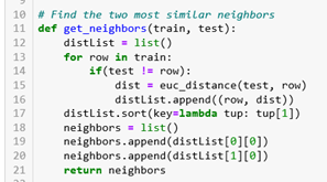
The next step is finding the most similar neighbors. As an input, the method takes a train – this is the dataset that the method should consider as a source for finding the nearest neighbors and a test parameter – this is a vector for which we need to find the neighbors. The method returns the two nearest neighbors for the requested test parameter. In this method, we are using the previously defined method for calculating the Euclidean distance and we will calculate the distance between the test parameter and the vectors contained in the train dataset. We will get only the first two values and return from this method.
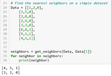
Now, we will use this method to find the nearest neighbors on a simple dataset that contains vectors. In this example, we are using the second vector [3,5,0] and we can see which vectors are the nearest neighbors for this one.
K means clustering
K-means clustering is a method of vector quantization, originally from signal processing, that aims to partition n observations into k clusters in which each observation belongs to the cluster with the nearest mean (cluster centers or cluster centroid), serving as a prototype of the cluster. This results in a partitioning of the data space into Voronoi cells. It is popular for cluster analysis in data mining. K-means clustering minimizes within-cluster variances (squared Euclidean distances), but not regular Euclidean distances, which would be the more difficult Weber problem: the mean optimizes squared errors, whereas only the geometric median minimizes Euclidean distances.
In other words, the K-means algorithm identifies k number of centroids, and then allocates every data point to the nearest cluster, while keeping the centroids as small as possible.
The example is in PySpark and after the implementation in PySpark, we can try with Python – just to visualize the results.
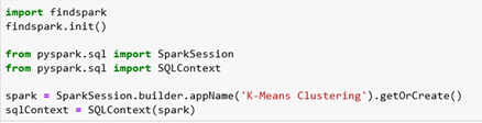
First, we will import the required packages. Since we are using PySpark, we need to initialize a spark session.
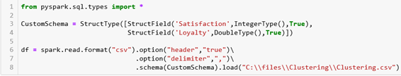
The next step is reading the CSV file – in this example, we have a simple dataset that contains information about the loyalty and satisfaction of customers. We will use a custom schema when reading the file.
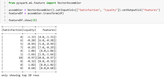
By using Vector Assembler which allows us to combine multiple vectors in one, we will define the features – in this case, we have two features that will be used. We can see that now our new dataset contains one new column called features.
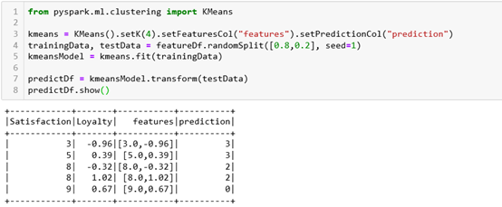
Now, we will use KMeans from PySpark. In this example, we will use 4 centroids and the dataset will be split in a way that 80% of the data will be for training and 20% for testing. In the picture below, we can see how our data in the test set is divided into clusters and which data points belong to which cluster.
Let’s try the same example in Python. First, we will scale the values in our dataset.

It is always a question of how to choose the appropriate number of centroids. In K-means clustering, the most important thing is to minimize the distance between points in a cluster and maximize the distance between clusters. These two things are dependent – if we minimize the distance between points, we automatically maximize the distance between clusters. The distance between points in a cluster is called ‘within-cluster sum of squares’ or shortly WCSS. If WCSS is minimized to be as low as possible, we have reached the perfect clustering solution. If we plot the WCSS with the number of clusters, we will get a plot that gives us information about the number of clusters appropriate for the dataset.

It looks like an elbow and that is why this method is called the “Elbow Method”. We can see that at the beginning the WCSS is declining extremely fast and at some point, is reaching an elbow. For our case, we can not determine the perfect solution – so we can try with 2, 3, 4, 5, and 9 clusters.
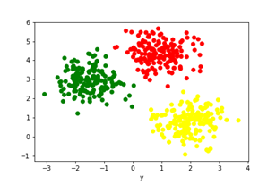
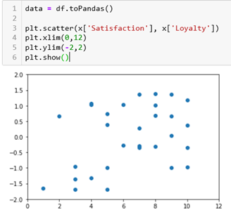
If we plot our dataset we can see how it is distributed:
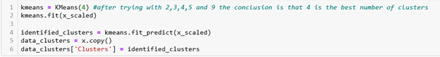
After trying with the number of clusters mentioned above, the conclusion was that 4 clusters are the best solution.
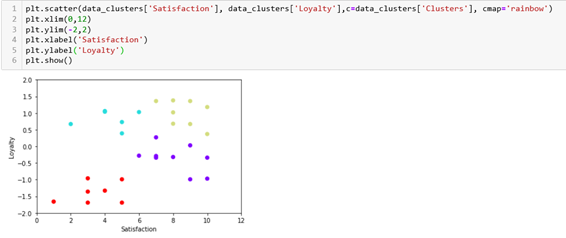
We will plot the results and we can see that our clusters make sense. We have customers that are not loyal and that are not satisfied, customers that are not loyal but are satisfied, customers that are loyal, but not satisfied, and customers that are both loyal and satisfied.

Conclusion
These are some basic algorithms that it is good to be familiar with if we want to work and gain an advantage while working with big datasets. There are more algorithms and we can say that each one of them has some advantages and usage. Working with big data is very challenging, but also very useful and helpful for organizations in making more intelligent decisions. We need to understand the data, analyze it, and extract the most important information insights. Choosing the right approaches and algorithms can help us in the process for sure.