

⋮IWConnect deals with Data Warehouse related projects and we provide a wide range of ETL (Extract Transform Load) services for warehouse data provisioning.
The purpose of this article is to demonstrate the basic concepts of using the SnapLogic platform for ETL dimension loading.
About SnapLogic
SnapLogic is an elastic integration solution that provides Integration Platform as a Service (iPaaS) tools for connecting Cloud data sources, SaaS applications, and on-premises business software applications. SnapLogic platform enables users to build, deploy, and efficiently manage multiple high-volume and data-intensive integration projects more quickly.
As an experienced SnapLogic Integration Consultancy partner, ⋮IWConnect has used SnapLogic for building integration solutions for external partners and clients, in a period of several years. Our experience with SnapLogic ranges in providing custom solutions applicable in a wide variety of industries including Telecommunications, Retail, Education, etc., with a focus on different types of integration like batch processing for ETL and big data management, as well as real-time API processing.
One of the goals we accomplished in the field of data integration is using the SnapLogic platform as an ETL tool in order to build a data warehouse in Amazon Redshift.
About AWS/Amazon Redshift
AWS or Amazon Web Services is a secure cloud services platform, offering compute power, database storage, content delivery, and other functionalities to help businesses scale and grow. Amazon Redshift is one of the cloud-based Amazon Web Services, which is a fast, fully managed petabyte-scale data warehouse service in the cloud.
SnapLogic offers a wide range of tools for integration with Amazon Redshift building the Snap pack that enables customers to transfer large amounts of data into and out of Amazon Redshift. The data can be moved at any latency (batch, read-time, real-time, and via triggers) to meet the requirements of a diverse set of business users.
In addition, SnapLogic supports connectivity to over 300 different data sources including connectors to cloud-based and on-premise systems that allow the accomplishment of the main goal – to easily extract data from various sources and format and load it into Amazon Redshift. We also have a possibility of developing custom connectors for other systems and additional features for the existing ones.
⋮IWConnect offers several custom solutions based on the SnapLogic ETL support:
- SnapLogic allows fast and easy ingesting, preparing, and delivering data
- Process and store massive volumes and varieties of data
- Feeding, reading, and analyzing large amounts of structured, complex, or social data
- Communication between a variety of data engines with a high percentage of reusability for different data platforms
- Focused on data streams between applications differentiated by its flexibility to connect to both cloud and on-premise systems
- Automation of end-to-end communication and many others.
In continuation, we’ll show an example of using SnapLogic as an ETL tool.
Problem:
There is a need to transfer data from an on-premise SQL server source in Amazon Redshift. One of the source tables applies to persons as a set of employees hired by a telecommunication company that works in a field providing technical services for customers. In Amazon Redshift, we need to design a dimension table representing technicians and a historical table with SCD (Slowly changing dimension) functionality applied.
SCD provides the functionality of storing and managing both current and historical data over time and resolves the problem by applying analytics and statistics on a historical basis. For example, there are fact tables that store records about work trips of employees who work on a field as a part of specifically evaluated work teams. The fact table is related to a dimension table that contains information about each employee. For historical reporting purposes, there might be a need to check the statistics about specific trips for an employee group in some period in the past that might not be identical to the current state. With SCD applied, both historical and current data are available at any point in time.
There are 6 basic types of SCD (referred to as type 0 through 6):
- Type 0– The passive method
- Type 1– Overwriting the old value
- Type 2– Creating a new additional record
- Type 3– Adding a new column
- Type 4– Using historical table
- Type 6– Combine approaches of types 1,2,3 (1+2+3=6)
Choosing the correct SCD type is very important and depends on the specific data conditions and structure, changing behavior, the business, etc.
To solve this particular problem, we are going to use the SCD type 2 method. This method provides tracking historical data by creating multiple records for a given natural key in the dimensional tables. History tracking is enabled using separate surrogate keys and different versions of the specific object. For example, if an employee relocates to another team, the version numbers will be incremented sequentially:
Another method is to track changes by date columns:
When using a combination of effective date and versioning information, the version number might be 1 for the current record and 0 for all historical records, while the schedule might be retrieved from date information.
The structure looks like in the example below:
Solution:
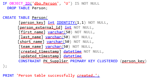
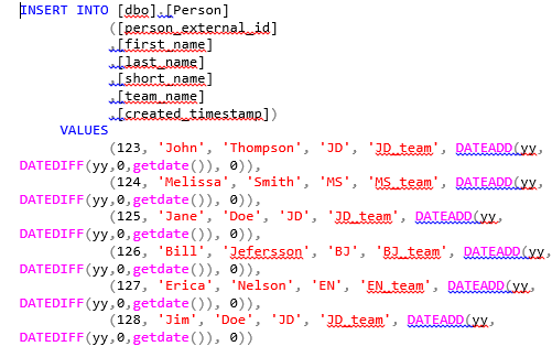
For this walkthrough, we need a source table called Person. We can run the following command to create a table named Person in the SQL server:
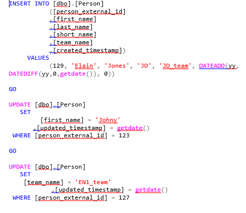
Then, we’ll populate the Person table with test data using the following insert script:
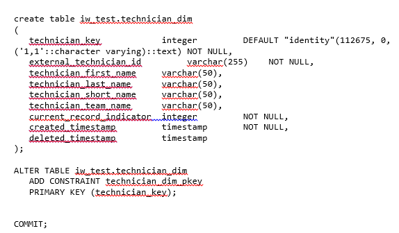
In parallel, we’ll need a dimension table in Redshift to transfer personal data, considering that every person is a technician who works in a field. The table will be named technician_dim.
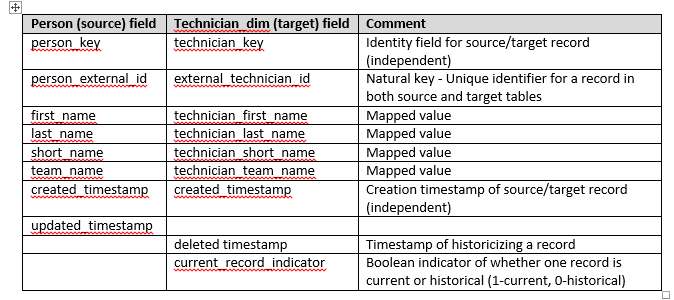
Mapping from the source to the target table is below:
Technician_dim table on Redshift is created using the following command:
As previously mentioned, we are going to use the SnapLogic platform as an ETL tool for loading data into Amazon Redshift, data maintenance, as well as detecting changes, and keeping data synchronized.
Compared to using an approach without a handy platform like SnapLogic, this process is much more complex and time-consuming. In short, the following actions will be needed:
- Upload the data files from all integrated systems and applications to an Amazon S3 Bucket to have them available for loading in specific tables.
- Run the COPY/INSERT Commands – Data is added in Amazon Redshift tables either by using an INSERT command or by using a COPY command. COPY command is many times faster and more efficient than INSERT commands.
- Create additional tables and processes for tracking changes, enabling historicization, merging data, etc. based on specific implementation designs.
- Vacuum and Analyze the database – to recover the space from deleted rows and restore the sort order and command updates on the statistics metadata, which enables the query optimizer to generate more accurate query plans.
All these steps with SnapLogic platform are available as a part of prebuilt connectors, and setting complex sophisticated process can be done very fast and much easier with configuration and adjustment of several settings.
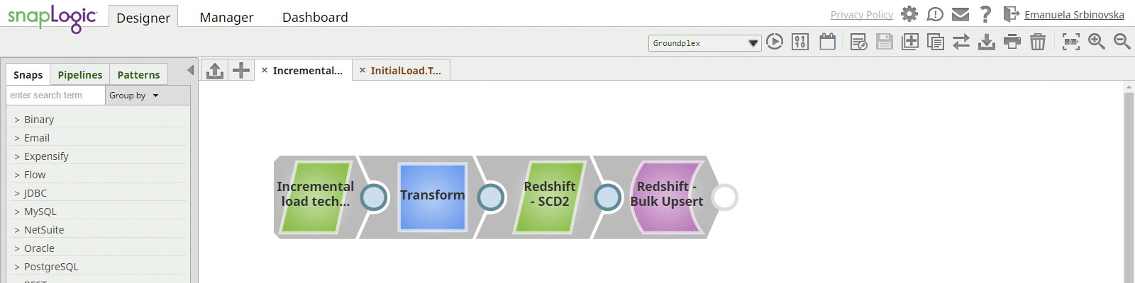
In SnapLogic, we will construct a simple pipeline for initial load of technician_dim table. In initial load pipeline we need to pool full data set from SQL server. The pipeline is consisted of three connectors/steps:
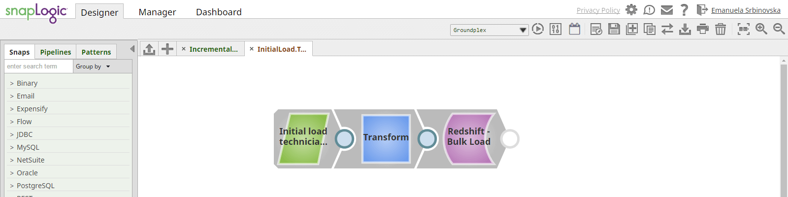
- SQL server select – select full data set from SQL server Person table
- Transform data and map it to the Redshift table structure
- Redshift Bulk Load – execute a Redshift bulk load operation. The input data is first written to a staging file on S3 and then the Redshift copy command is used to insert data into the target technician_dim table (automatically done by the snap).

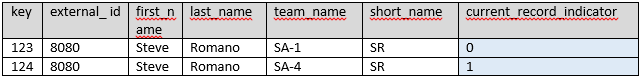
After completing bulk load operation, we have full data set loaded in technician_dim table:
Now we can consider that initial data set is loaded in Redshift table. The next thing we need to do is to create incremental (delta) load pipeline in SnapLogic for the next data loads that will capture changes in the source table and mark a record as historical if needed.
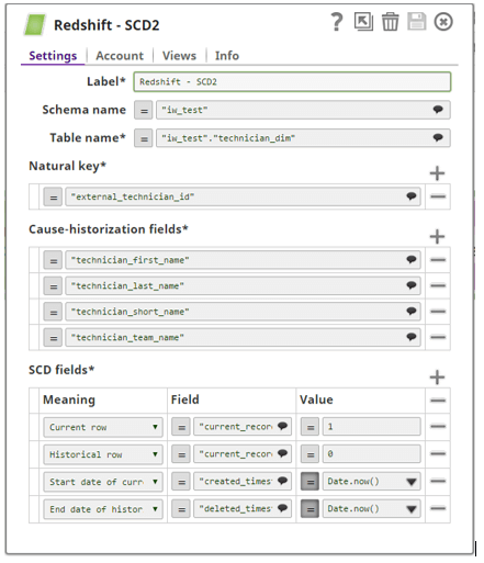
SnapLogic offers a snap SCD2 that provides functionality of SCD (Slowly changing dimension) Type 2 on target Redshift table. As technician_dim table is designed to be historical table, we are going to use this functionality to provide tracking of the records.
Name fields of the source table will be used to cause – historization fields. The natural key will be person_external_id field.
In order to force record historization in the target dimension table, we need to trigger changes in source data.
For example, we’re going to insert one new record and update two of the existing records by executing following SQL scripts on Person table in SQL server:
The example below describes how the Redshift – SCD2 Snap can be used.
- SQL server select – select only new and updated records from SQL server Person table.
- Transform data and map it to the Redshift table structure
- Cause SCD type 2 – Redshift SCD2 snap executes one SQL lookup request per multiple input documents to avoid making a request for every input record. The Snap produces a stream of documents for Redshift Bulk Upsert Snap to update or insert rows into the target table. Therefore, this Snap should be connected to Redshift Bulk Upsert Snap in the pipeline in order to accomplish a complete SCD2 functionality.
Configuration of SCD2 snap is as follows:
- Natural key – unique identifier per row (entity) in the target table
- Cause-historization fields – names of fields of which any change in values causes historization of an existing row and insertion of new current row in the target table
- SCD fields
- Current row – set value of the field which identifies current record. In our case that is ‘current_record_indicator’ and its value is set to 1.
- Historical row – set value of the field which identifies historical record. In our case that is ‘current_record_indicator’ and its value is set to 0.
- Start date of current row
- End date of historical row
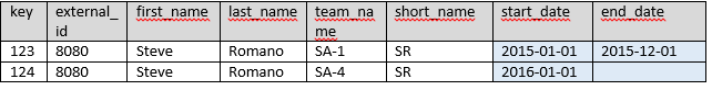
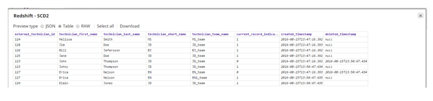
Using this configuration, output of the SCD2 snap will be as follows:
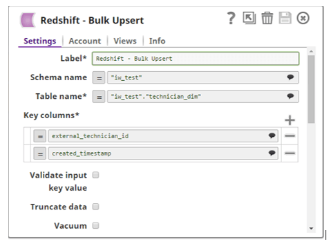
4. Redshift Bulk Upsert – depending on SCD2 snap input, rows will be inserted and/or updated in the target table if any change is captured in incoming documents. In the configuration settings, we have to specify key columns, consisted of a combination of natural key and start date field:
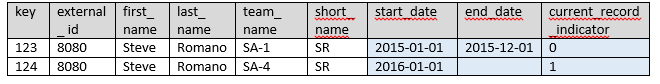
After running the pipeline, the state of technician_dim table is as follows:
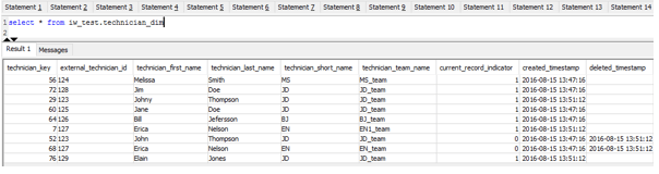
We can confirm the three changes captured in the pipeline:
- New record is inserted (technician_key = 76)
- The record where technician_key = 68 is historicized and new record is inserted for the same person (with technician_key = 7).
- The record with technician_key = 52 is historicized and new record is inserted for the same person (with technician_key = 29).
Conclusion
SnapLogic offers the capability to integrate Amazon Redshift data with any other data sources in the cloud, on premise or in hybrid mode, with the following advantages:
- Do sophisticated extract, transform and load (ETL) operations such as slowly changing dimension type 2 (SCD2) and database lookups without any custom coding in a short design and development time.
- Accelerate cloud data warehouse adoption with prebuilt patterns that can be configured by an automatically-generated series of steps.
- Rapidly connect Amazon Redshift to a variety of relational database services including SQL Server, Amazon RDS for MySQL, PostgreSQL, Oracle etc.
- Quickly load data into an Amazon S3 bucket and kick off the Amazon Redshift import process in a single step.
- Easily detect daily changes to keep data synchronized.
- Visually design a variety of data operations and transform actions using a wide set of core snaps.
- Directly connect to many existing BI tools such as Tableau, Birst and Anaplan, reducing the time to convert raw data into actionable insights.